How to Use XLOOKUP in Excel: A Practical Guide with Examples

If you’ve spent any time working with Excel formulas, you’ve probably used VLOOKUP at some point. It gets the job done, but it comes with a list of frustrations: it only looks right, it breaks when you insert columns, and returning multiple results takes ugly workarounds. How to use XLOOKUP in Excel solves most of those problems with a cleaner, more flexible function. This guide covers the XLOOKUP formula from scratch, with real examples, multiple criteria techniques, and a clear comparison of XLOOKUP vs VLOOKUP so you know when to use which.

What Is XLOOKUP?

The XLOOKUP function in Excel was introduced in 2019 as a modern replacement for VLOOKUP, HLOOKUP, and INDEX/MATCH. It’s available in Excel 365 and Excel 2021. If you’re on Excel 2016 or 2019 (non-365), XLOOKUP is not available. In that case, INDEX/MATCH is your best alternative.

XLOOKUP is a lookup function in Excel that searches a range or array for a value and returns a corresponding result from another range or array. Unlike VLOOKUP, it can search both left and right, works with rows and columns equally, and handles errors gracefully with a built-in “if not found” argument.

The XLOOKUP Formula: Syntax Explained

The basic XLOOKUP formula looks like this:

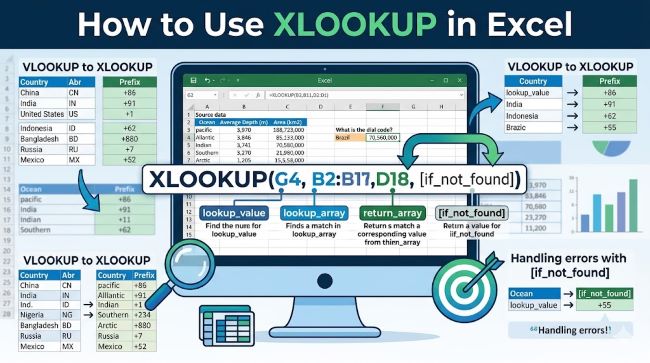
=XLOOKUP(lookup_value, lookup_array, return_array, [if_not_found], [match_mode], [search_mode])

Breaking down each argument:

lookup_value: The value you’re searching for. This can be a cell reference, a value, or a text string in quotes.
lookup_array: The range or column where you want Excel to search for the lookup_value.
return_array: The range or column from which Excel should return the result.
[if_not_found]: Optional. Text to display if no match is found. If omitted, Excel returns a standard #N/A error.
[match_mode]: Optional. 0 = exact match (default), -1 = exact or next smaller, 1 = exact or next larger, 2 = wildcard match.
[search_mode]: Optional. 1 = search from first to last (default), -1 = search from last to first, 2 = binary search ascending, -2 = binary search descending.

The first three arguments are required. The last three are optional and cover most edge cases you’ll encounter.

Basic XLOOKUP Example

Say you have a table with employee IDs in column A and employee names in column B. You want to look up an ID and return the name.

Table:

A (ID)	B (Name)
1001	Sarah
1002	Marcus
1003	Li Wei

Formula in cell D2:

=XLOOKUP(D1, A2:A4, B2:B4, "Not found")

If D1 contains 1002, this returns “Marcus.” If D1 contains 9999, this returns “Not found” instead of an error.

This is the most common use case. Clean, readable, and no column index number required.

XLOOKUP vs VLOOKUP: The Key Differences

The difference between XLOOKUP and VLOOKUP comes down to flexibility and reliability.

VLOOKUP limitations:

Searches only left-to-right. The lookup column must be the leftmost column in your range.
Requires a column index number that breaks when you insert or delete columns.
Returns the first match only with no built-in error handling.
Slower on large datasets.

XLOOKUP advantages:

Searches in any direction: left, right, up, or down.
Uses separate lookup and return arrays, so column insertions don’t break the formula.
Built-in “if_not_found” argument handles missing values cleanly.
Can return multiple columns at once by selecting a multi-column return_array.
Faster on large datasets with the binary search mode.

XLOOKUP vs VLOOKUP example: In VLOOKUP, if your lookup column is column C and you want to return something from column A (to the left), you can’t do it without adding helper columns or using INDEX/MATCH. With XLOOKUP, you simply point the return_array at column A and it works.

The only reason to still use VLOOKUP in 2026 is backward compatibility. If you share spreadsheets with people on Excel 2016 or older, XLOOKUP formulas will break for them. In that context, sticking to VLOOKUP or INDEX/MATCH is the safer choice. Choosing the right office suite and version for your team matters more than most people realise when it comes to formula compatibility across collaborators.

XLOOKUP Multiple Criteria

Using XLOOKUP multiple criteria requires a small trick: concatenate your criteria into a single lookup value and do the same in the lookup array.

Scenario: You have a table with Region in column A, Product in column B, and Sales in column C. You want to find sales for “East” region and “Widget A” product.

Formula:

=XLOOKUP(F1&G1, A2:A100&B2:B100, C2:C100, "Not found")

This concatenates “East” and “Widget A” into “EastWidget A” and searches the combined A&B array for the same string. When a row in A&B matches both conditions simultaneously, XLOOKUP returns the corresponding value from column C.

Important: This is an array formula. In Excel 365, it works without pressing Ctrl+Shift+Enter. In older Excel versions with XLOOKUP support (Excel 2021), it also works as a regular formula.

For more complex multi-criteria scenarios, you can nest XLOOKUP inside IF or use FILTER as an alternative.

Returning Multiple Columns with XLOOKUP

One of the most useful features of the XLOOKUP excel function is the ability to return more than one column at once. Simply expand the return_array to cover multiple columns.

Example: Return both Name and Department from a lookup:

=XLOOKUP(A2, EmployeeID_range, B2:C100, "Not found")

This returns a dynamic array that spills into adjacent cells automatically, filling in both columns from a single formula. This is a feature unique to Excel 365’s dynamic array engine and makes dashboards and summary tables significantly easier to build.

How to Use XLOOKUP for Reverse Lookup

Since XLOOKUP can search in any direction, reverse lookups (returning a value to the left of the lookup column) are straightforward.

Example: Name is in column A, ID is in column B. Find the ID for a given name:

=XLOOKUP("Marcus", B2:B100, A2:A100, "Not found")

Lookup column B for “Marcus,” return from column A. No helper columns, no workarounds.

XLOOKUP for Approximate Match

The [match_mode] argument handles approximate matches.

Use -1 to return the next smaller value when an exact match isn’t found. Useful for tax brackets, commission tiers, or price bands.
Use 1 to return the next larger value. Useful for minimum thresholds.

Example for tiered pricing:

=XLOOKUP(D2, TierThresholds, TierPrices, "Below minimum", -1)

If D2 = 750 and your tiers are 500, 1000, 2000, this returns the price for the 500 tier (next smaller value below 750).

XLOOKUP Google Sheets: Is It Available?

XLOOKUP Google Sheets support is limited. Google Sheets does not have a native XLOOKUP function as of 2026. Google’s equivalent is a combination of VLOOKUP, INDEX/MATCH, or the XLOOKUP-like functionality provided through the newer XMATCH and XLOOKUP that Google has been rolling out gradually to Workspace accounts.

If you need XLOOKUP-style functionality in Google Sheets right now, INDEX/MATCH is the most reliable alternative:

=INDEX(return_range, MATCH(lookup_value, lookup_range, 0))

This matches XLOOKUP’s core functionality (including left-side lookups) without requiring the XLOOKUP function. Google Workspace add-ons and extensions can also extend Sheets’ formula capabilities, though they don’t add XLOOKUP natively.

Common XLOOKUP Errors and Fixes

#N/A error: No match found and no [if_not_found] argument specified. Add a fourth argument: =XLOOKUP(A2, range1, range2, "Not found").

#VALUE! error: The lookup_array and return_array have different sizes. Make sure they cover the same number of rows.

Spill error (#SPILL!): Something is blocking the cells where XLOOKUP wants to place its results. Clear the cells in the spill range.

Wrong result returned: Check whether [match_mode] is set correctly. The default is exact match (0). If you’re getting unexpected approximate matches, confirm the argument.

XLOOKUP for Data Analysis Beyond Basic Lookups

As your spreadsheet work becomes more complex, XLOOKUP becomes one piece of a larger data analysis toolkit. Pairing it with FILTER, SORT, UNIQUE, and dynamic array formulas builds genuinely powerful reporting without needing pivot tables for every question. For even larger scale data work that goes beyond what Excel handles efficiently, dedicated business intelligence tools handle the aggregation and relationship mapping that lookup functions approach but can’t fully replace.

Key Takeaways

How to use XLOOKUP in Excel: =XLOOKUP(lookup_value, lookup_array, return_array, [if_not_found], [match_mode], [search_mode]). The first three arguments are required.
XLOOKUP vs VLOOKUP: XLOOKUP searches in any direction, doesn’t break on column insertions, handles errors natively, and can return multiple columns. Use VLOOKUP only for backward compatibility with older Excel versions.
Difference between XLOOKUP and VLOOKUP: VLOOKUP requires the lookup column to be leftmost. XLOOKUP has no such restriction.
XLOOKUP multiple criteria: concatenate criteria in both the lookup_value and lookup_array using the & operator.
XLOOKUP formula for approximate match: use -1 in match_mode to return the next smaller value, or 1 for next larger.
XLOOKUP Google Sheets: not natively available as of 2026. Use INDEX/MATCH as the equivalent.
XLOOKUP function in Excel requires Excel 365 or Excel 2021. It is not available in Excel 2016 or 2019 (non-subscription).
Use the [if_not_found] argument in every formula to avoid #N/A errors in your worksheets.