How to Freeze a Row in Excel: Complete Step-by-Step Guide

Freezing a row in Excel is one of the most useful features for working with large datasets. When you scroll down through hundreds or thousands of rows, your column headers disappear and you lose track of what each column represents. Freezing the top row keeps those headers visible no matter how far down you scroll. This guide covers every variation: freezing the top row, freezing multiple rows, freezing columns, freezing both rows and columns together, and how to unfreeze when you’re done.

How to Freeze the Top Row in Excel

This is the most common use case and the fastest to apply.

Step 1: Open your Excel workbook and navigate to the worksheet where you want to freeze the header row.

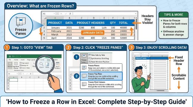
Step 2: Click the View tab in the ribbon at the top of the screen.

Step 3: In the Window group, click Freeze Panes.

Step 4: From the dropdown menu, select Freeze Top Row.

That’s it. A thin dark line appears below row 1 to indicate it’s frozen. Now scroll down and row 1 remains fixed at the top of the screen while all other rows scroll normally beneath it.

This method always freezes row 1 regardless of where your active cell is. If your headers are in row 1 (which is the standard layout), this is the method to use.

How to Freeze Multiple Rows in Excel

If your spreadsheet has a multi-row header (row 1 contains a title, row 2 contains column headers, for example) or you want to freeze more than one row, the process is slightly different.

Step 1: Click on the row number of the first row you want to be scrollable. In other words, click the row directly below the last row you want frozen. If you want rows 1 and 2 frozen, click on row 3.

Step 2: With that row selected (or with your active cell in column A of that row), go to the View tab.

Step 3: Click Freeze Panes.

Step 4: Select Freeze Panes (the first option in the dropdown, not “Freeze Top Row”).

A dark line appears below the last frozen row. Everything above that line stays fixed when you scroll down.

The key principle: Excel freezes everything above and to the left of the selected cell. To freeze rows only, click the cell in column A of the first row you want to scroll. To freeze a specific number of rows, count down to the row after your last header row and click there.

How to Freeze a Column in Excel

The same Freeze Panes feature handles columns. To freeze the leftmost column:

Step 1: Go to View > Freeze Panes > Freeze First Column.

A thin line appears to the right of column A, and it stays visible while you scroll right.

To freeze multiple columns, click the cell at the top of the first column you want to scroll (e.g., click cell C1 to freeze columns A and B), then go to View > Freeze Panes > Freeze Panes.

How to Freeze Both a Row and a Column Simultaneously

To freeze row 1 and column A at the same time:

Step 1: Click cell B2. This is the cell directly below row 1 and to the right of column A.

Step 2: Go to View > Freeze Panes > Freeze Panes.

Both row 1 and column A will be frozen. A dark line appears below row 1 and to the right of column A. Now when you scroll right, column A stays visible. When you scroll down, row 1 stays visible.

To freeze two rows and two columns simultaneously, click cell C3 (the cell below row 2 and to the right of column B) and apply Freeze Panes.

How to Unfreeze Rows in Excel

To remove any freeze you’ve applied:

Step 1: Go to the View tab.

Step 2: Click Freeze Panes.

Step 3: The first option in the dropdown will now say Unfreeze Panes (it changes from Freeze Panes once any freeze is active). Click it.

All frozen rows and columns are immediately released. The dark dividing lines disappear.

Note: you don’t need to select anything specific before unfreezing. The Unfreeze Panes option removes all active freezes on the sheet at once.

Common Problems with Freezing Rows

“Freeze Top Row” is greyed out or missing. This happens when the workbook is in Page Layout view rather than Normal view. Go to View > Normal to switch back to Normal view, then freeze panes will be available.

The freeze line appears in the wrong place. Freeze Panes (the first option) freezes based on your active cell position. If the freeze line is in the wrong place, unfreeze and reselect the correct cell before applying again.

Can’t freeze rows because the sheet is protected. Sheet protection can prevent changes to frozen panes. Go to Review > Unprotect Sheet before attempting to freeze.

Frozen row doesn’t appear when printing. Freeze Panes is a display feature only: it affects how the sheet looks on screen but not how it prints. To repeat header rows on every printed page, go to Page Layout > Print Titles > Rows to repeat at top and select your header row there.

Freeze Panes vs. Split

Excel also has a Split feature (View > Split) that divides the worksheet window into independent scrollable panes. Unlike frozen panes, both sections in a split can scroll independently. Freeze panes is better for keeping headers visible. Split is better when you need to compare two distant sections of the same sheet simultaneously.

For other Excel skills that pair with knowing how to freeze a row in Excel, how to unhide all rows in Excel covers another common row management task, and how to create a drop down list in Excel helps you build more structured spreadsheets where frozen headers and validated inputs work together.

Key Takeaways

To freeze the top row in Excel: View > Freeze Panes > Freeze Top Row. A dark line appears below row 1 confirming the freeze
To freeze multiple rows: click the cell in column A of the first row you want to scroll, then go to View > Freeze Panes > Freeze Panes
The rule: Excel freezes everything above and to the left of the selected cell when you apply Freeze Panes
To freeze a row and column simultaneously: click the cell one row below and one column to the right of your freeze point (e.g., B2 to freeze row 1 and column A)
To unfreeze: View > Freeze Panes > Unfreeze Panes. The option name changes once a freeze is active
Freeze Panes is a display feature only and does not affect printing: use Page Layout > Print Titles to repeat headers on printed pages
If Freeze Panes is greyed out, switch from Page Layout view to Normal view using View > Normal