
How to Create a Drop Down List in Excel: Step-by-Step Guide
A drop down list in Excel restricts what users can enter in a cell to a predefined set of options. This reduces data entry errors, speeds up input, and keeps your spreadsheets consistent. Whether you’re building a budget tracker, a project management tool, or a data entry form, knowing how to create a drop down list in Excel is one of the most practical skills in the application. This guide covers every method from the simplest manual approach to dynamic lists that update automatically.
Method 1: Create a Drop Down List with Manually Typed Items
This is the quickest approach when your list of options is short and unlikely to change.
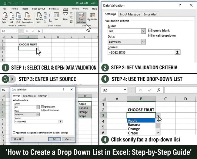
Step 1: Click the cell or select the range of cells where you want the drop down list to appear.
Step 2: Go to the Data tab in the ribbon.
Step 3: Click Data Validation in the Data Tools group.
Step 4: In the Data Validation dialog box, click the Settings tab.
Step 5: In the Allow dropdown, select List.
Step 6: In the Source field, type your items separated by commas. For example: Yes,No,Maybe or Pending,In Progress,Complete,Cancelled.
Step 7: Make sure In-cell dropdown is checked.
Step 8: Click OK.
The cell now shows a small dropdown arrow when selected. Click the arrow to see and choose from your list options.
Method 2: Create a Drop Down List from a Cell Range
When your list is longer or you want to be able to update the options without editing the validation settings, reference a range of cells instead of typing items manually.
Step 1: Enter your list items in a column somewhere in your workbook. For example, put Yes, No, and Maybe in cells E1, E2, and E3. You can put this list on a separate sheet to keep it out of the way.
Step 2: Select the cell or range where you want the drop down list.
Step 3: Go to Data > Data Validation > Settings.
Step 4: Set Allow to List.
Step 5: In the Source field, instead of typing items, click the range selector icon and select your list range (e.g., E1:E3). Or type the range reference directly: =$E$1:$E$3.
Step 6: Click OK.
Now when you update the items in E1:E3, the drop down list automatically reflects the changes without reopening Data Validation.
Method 3: Use a Named Range for Cleaner References
Named ranges make your dropdown formula cleaner and easier to maintain, especially when the source list is on a different sheet.
Step 1: Select the cells containing your list items.
Step 2: Click the Name Box (the cell reference box to the left of the formula bar) and type a name for the range, for example StatusOptions. Press Enter.
Step 3: Select the cell where you want the drop down list.
Step 4: Go to Data > Data Validation > Settings, set Allow to List, and in the Source field type =StatusOptions.
Step 5: Click OK.
Named ranges are particularly useful when you create a drop down list in Excel that references a list on another sheet, since cross-sheet references like =Sheet2!$A$1:$A$10 work in Data Validation but named ranges are simpler to read and maintain.
Method 4: Create a Dynamic Drop Down List (Updates Automatically)
A standard range reference doesn’t automatically expand when you add items to the list. A dynamic drop down list solves this using an Excel Table or the OFFSET function.
Using an Excel Table (recommended, simplest):
Step 1: Select your list items and press Ctrl + T to convert them into an Excel Table. Give the table a name (e.g., OptionsList) in the Table Design tab.
Step 2: Create a named range that refers to the table column. Go to Formulas > Name Manager > New. Name it (e.g., DynamicOptions) and in the Refers To field enter: =OptionsList[Column1] (replacing Column1 with your actual column header name).
Step 3: Use =DynamicOptions as the source in your Data Validation settings.
Now when you add items to the bottom of your Excel Table, they automatically appear in the drop down list.
Adding Input Messages and Error Alerts
The Data Validation dialog has two additional tabs worth using:
Input Message tab: Set a title and message that appears when the user clicks the cell. For example: “Select a status” with message “Choose from the options in the dropdown.” This guides users filling out the sheet.
Error Alert tab: Controls what happens when someone types a value not in your list.
- Stop: prevents the entry entirely (strictest)
- Warning: shows a warning but allows the user to proceed
- Information: shows a note but doesn’t interfere
For shared spreadsheets where data consistency matters, using Stop with a clear error message helps maintain clean data.
How to Apply a Drop Down List to Multiple Cells
To apply the same drop down list to an entire column or a range:
Step 1: Select the full range before opening Data Validation (e.g., click B2 and drag to B100, or click the column header B to select the entire column).
Step 2: Apply Data Validation as described above.
All cells in the selection will have the same drop down list. You can also copy a cell that already has Data Validation and paste it using Paste Special > Validation (Alt + Ctrl + V, then choose Validation) to apply just the validation without overwriting other cell content.
How to Edit or Remove a Drop Down List
To edit: select a cell with the drop down list, go to Data > Data Validation, and modify the Source or other settings. To apply the same change to all cells with the same validation, check Apply these changes to all other cells with the same settings at the bottom of the dialog before clicking OK.
To remove: select the cell(s), go to Data > Data Validation, and click Clear All in the bottom-left of the dialog, then click OK. The validation is removed and the cell accepts any input again.
Dependent Drop Down Lists (Cascading Lists)
A dependent drop down list changes its options based on the selection in another cell. For example, selecting “Fruit” in one cell makes the next dropdown show Apple, Banana, Mango, while selecting “Vegetable” shows Carrot, Broccoli, Spinach.
This uses named ranges matching the category names combined with the INDIRECT function in the Source field: =INDIRECT(A2) where A2 contains the category selection. Each category name must match a named range exactly for INDIRECT to work.
For other Excel skills that work well alongside knowing how to create a drop down list in Excel, how to freeze a row in Excel keeps your headers visible while users scroll through long data entry forms, and how to unhide all rows in Excel is useful when troubleshooting sheets built by others.
Key Takeaways
- Create a drop down list in Excel via Data > Data Validation > Settings > Allow: List, then enter items manually in Source (comma-separated) or reference a cell range
- Range-based lists (referencing cells rather than typing items) are easier to update: change the source cells and the dropdown updates automatically
- Named ranges make cross-sheet references cleaner: name your list range and use
=RangeNamein the Source field - Convert your source list to an Excel Table for a truly dynamic drop down list that expands automatically when you add new items
- Use the Error Alert tab set to Stop to prevent users from typing values not in your list, maintaining data consistency in shared workbooks
- To apply dropdown validation to multiple cells, select the full range before opening Data Validation
- Dependent (cascading) dropdowns use named ranges plus the INDIRECT function to change dropdown options based on another cell’s value


