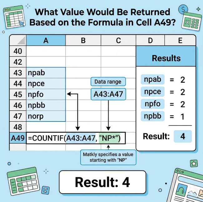
Understanding Excel Formulas: What Value Would Be Returned Based on the Formula in Cell A49

You’re working in a spreadsheet, staring at a cell, and wondering what value would be returned based on the formula in cell A49. Maybe you inherited a workbook from someone else. Maybe you’re trying to audit a calculation. Or maybe you’re just curious about how Excel evaluates a specific formula before you run it. This happens more often than people realize, and it’s a legitimate question that separates users who understand spreadsheet logic from those who just type numbers in.

The answer to what value would be returned in Excel A49 depends entirely on what formula sits in that cell and what data it references. That’s the honest answer. But the real value is understanding how to figure it out yourself, trace the logic, and verify the result before you trust it.

How Excel Formulas Work

Excel formulas are instructions. When you enter a formula into a cell, Excel doesn’t store the formula itself as the display value. It calculates the result and shows you the outcome. The formula bar at the top shows what’s actually in the cell. The spreadsheet shows what the formula produces.

This distinction matters because when someone asks what value would be returned based on the formula in cell A49, they’re really asking two things: What does the formula do, and what inputs does it use.

The Basic Calculation Process

Let’s say cell A49 contains =SUM(A1:A48). The value returned would be the sum of all cells from A1 to A48. If those cells contain 10, 20, and 30 (with the rest empty), the result is 60. Simple. But if you change one of those cells to 40, the result updates instantly to 70.

That’s the beauty and the occasional frustration of spreadsheets. Formulas are dynamic. They recalculate whenever their inputs change.

Common Formula Types in Spreadsheets

Different formulas return different types of values. Understanding the formula type tells you what kind of result to expect.

• SUM formulas add numbers together. They return a numeric total.
• AVERAGE formulas calculate the mean of a set of numbers. They return a decimal or whole number depending on your data.
• COUNT formulas count how many cells contain numbers. They return a count, always a whole number.
• IF formulas return one value if a condition is true, another if it’s false. They can return text, numbers, or even other formulas.
• VLOOKUP formulas find a value in one column and return a related value from another column. The value returned depends on your lookup table and search criteria.
• Text formulas like CONCATENATE combine text strings. They return combined text.

These are just the basics. Excel has hundreds of functions, and each one handles inputs and produces outputs differently.

Tracing Cell References and Precedents

Understanding Formula Dependencies

When you want to know what value would be returned in Excel A49, start by looking at what’s actually in that cell. Click on A49. Look at the formula bar. Read the formula.

Then trace the references. If the formula uses cells like A1, A2, or A50, look at those cells. What values do they contain? Are they numbers? Text? Other formulas?

Using Excel’s Trace Tools

Excel has a tool for this. Go to the Formulas tab and use Trace Precedents. This shows you with arrows which cells your formula depends on. It’s invaluable for understanding the chain of calculations, especially in complex spreadsheets.

If A49 depends on A48, and A48 depends on A47, you need to trace back through the chain. Sometimes the value returned depends on calculations that happened several steps earlier.

When Formulas Return Errors

Identifying Common Error Types

Sometimes what value would be returned is an error. Understanding these signals helps you fix problems:

• #REF! means the formula references a cell that no longer exists or is invalid.
• #VALUE! means the formula tried to perform an operation on data that doesn’t work for that operation. Adding text to a number can trigger this.
• #DIV/0! means the formula tried to divide by zero.
• #N/A means the formula couldn’t find what it was looking for. Usually seen with VLOOKUP or similar functions.
• #NAME? means Excel doesn’t recognize the function name or a named range the formula uses.

These errors are signals. They tell you something is wrong with either the formula itself or the data it’s trying to process. Don’t ignore them. Fix the underlying issue.

Evaluating Formulas Step by Step

Using the Formula Evaluator Tool

Excel has another helpful tool: the Formula Evaluator. It walks through your formula one piece at a time, showing you what each part calculates to.

Open the Formulas tab, click Evaluate Formula, and select your cell. Then click Evaluate repeatedly to step through the calculation. This shows you exactly where the formula goes and what intermediate values it produces.

This is especially helpful for complex formulas with nested functions. A formula like =IF(SUM(A1:A10)>100,AVERAGE(B1:B10),0) has multiple layers. The evaluator breaks it down so you can see SUM first, then the comparison, then which branch of the IF statement executes.

The Importance of Cell Formatting

How Formatting Affects Display vs. Value

Sometimes the value returned by a formula is correct, but it displays wrong. This happens with formatting.

If a cell contains the number 100 but you format it to show zero decimal places, it displays as 100. Format it to show two decimal places, and it displays as 100.00. The underlying value hasn’t changed, just how it displays.

Currency formatting can mask the true numeric value. Percentage formatting divides the number by 100. Date formatting turns numbers into dates. All of this happens at the display level. The actual value in the cell remains what the formula calculated.

This matters when you’re troubleshooting. Sometimes you think the formula is wrong, but it’s calculating correctly and displaying with unexpected formatting.

Named Ranges Make Formulas Clearer

Why Named Ranges Matter

When a formula uses named ranges instead of cell references, understanding what value would be returned becomes easier to read.

Instead of =SUM(A1:A48), you could have =SUM(QuarterlyRevenue). If you define QuarterlyRevenue as A1:A48, the formula does exactly the same calculation, but the intent is clearer.

Named ranges reduce errors too. You type the name instead of trying to remember which cells to reference. And if your data range expands, you update the named range once, and all formulas using it update automatically.

Consider using named ranges for any calculation you revisit or share with others. It makes auditing easier and formulas more maintainable.

Testing Formulas Before Relying on Them

Verification Strategies

Before you trust what value would be returned based on a formula, test it.

• Change one input value and verify the output changes appropriately. If A49 sums A1 through A48, increase one of those values by 10 and check that A49 increases by 10.
• Compare the result to a manual calculation if the data set is small. Use a calculator or rough math to verify.
• Look for outliers. If A49 should be around 500 but shows 50000, something is wrong.
• Use filters to see what data the formula includes. Sometimes formulas reference hidden rows or cells that contain zero or blank values. These can affect your result.
• Check the formula’s assumptions. Does it assume all data is numeric? Does it exclude header rows? Does it apply to the right date range?

Excel formulas are powerful, but they only work correctly if the logic is sound and the data is right.

How to Document Your Formulas

Creating Useful Documentation

When you create a formula that calculates something important, document it. Add a comment explaining what it does. Describe which cells it uses and why.

This helps you six months from now when you can’t remember what you were thinking. It helps colleagues understand your logic. It makes troubleshooting faster when something breaks.

You can add comments in Excel by right-clicking a cell and selecting New Comment. Write a brief explanation of the formula’s purpose and any assumptions it makes.

For complex calculations, consider creating a separate reference sheet that explains all your formulas. List the cell location, the formula, what it calculates, and any notes about data sources or updates. This approach complements solid web design practices that emphasize clear communication and documentation.

Linking Formulas Across Sheets

Managing Multi-Sheet Calculations

Sometimes what value would be returned in cell A49 depends on calculations on another sheet entirely. Excel handles this well.

A formula can reference another sheet using the syntax =SheetName!A49. This pulls the value from cell A49 on a different sheet. You can even link to cells in external workbooks if needed.

When formulas span multiple sheets, document the structure clearly. Create a map showing which sheets feed into which calculations. This prevents circular references and makes auditing much easier. Just as information architecture matters in web design, organizing your formula structure matters in spreadsheets.

Circular references occur when a formula references itself, directly or indirectly. Excel detects these and flags them. They prevent proper calculation, so fix them immediately.

Common Mistakes When Evaluating Formulas

Pitfalls to Avoid

People often misunderstand what a formula returns because of common mistakes.

• Forgetting to press Enter after typing a formula means Excel hasn’t calculated it yet. The formula bar shows your input, but the cell is still empty or shows the old value.
• Using relative instead of absolute references causes confusion. A49 might reference A1:A48 with relative references, so if you copy the formula, the references shift. Understanding which references are relative and which are absolute is crucial.
• Mixing data types causes errors. If A49 tries to add a text value to a number, it fails. Check that your data is consistently formatted.
• Not updating linked formulas means you get stale data. If A49 references an external file, make sure that file is current.
• Forgetting about calculation mode. By default, Excel recalculates automatically. But if you or someone else switched to manual calculation mode, formulas don’t update when data changes. Check this in the Formulas tab.

Verify Your Understanding

The best way to confirm what value would be returned based on the formula in cell A49 is to click the cell, read the formula, trace the references, evaluate step by step, and test with known inputs.

Don’t assume. Don’t guess. Verify. Excel gives you the tools to do this. Use them.

When you understand how a formula works, you understand your data. You can spot errors, find opportunities for improvement, and make better decisions based on accurate calculations. That’s the real value in asking the question in the first place.

Take time to learn how to read and evaluate formulas. It separates casual spreadsheet users from people who actually know what they’re doing. And in a world where data drives decisions, that matters more than you might think. Much like a mobile-first design approach ensures everyone can access information clearly, understanding your formulas ensures your data is accessible and reliable.

Key Takeaways

• The value returned by a formula in cell A49 depends on the formula itself and the data it references.
• Use the formula bar to see what formula is actually in the cell, not just the result.
• Trace precedents to understand which cells feed into your calculation.
• Use the Formula Evaluator to step through complex formulas and see intermediate values.
• Check for errors like #REF!, #VALUE!, and #DIV/0! which indicate problems with the formula or data.
• Test formulas with known inputs to verify they calculate correctly.
• Document your formulas so others (and your future self) understand what they do and why.
• Named ranges make formulas clearer and easier to maintain.
• Don’t forget that formatting affects how values display, not what they actually are.
• Circular references must be fixed immediately to ensure proper calculation.